Concept Drift Detection
Authors: India Lindsay, Thomas Schill, Leigh Nicholl
Concept drift is defined as changes in the properties of a model’s target variable that result in significant changes in the predictive ability of the model over time [1]. These drops in performance are the result of new concepts appearing in either the feature values, the true labels, or the relationship between the two.
Concept drift detection algorithms monitor a classifier’s performance metrics over time and alert users to changes in performance resulting from drift [2]. They might monitor a single performance metric, such as accuracy, or multiple metrics simultaneously, such as true positive, false positive, true negative, and false negative rates.
Concept drift detectors typically use the hypothesis testing framework to identify drift. The goal is to determine whether the data occurring at some timestamp, the “reference data,” is different from the data occurring at a later timestamp, the “test data.” A concept drift algorithm defines a test statistic, based on the performance metric it is monitoring, to summarize the differences between these two. The null hypothesis states that the reference and test data share a common probability distribution, while the alternative hypothesis states that they do not. If the value of test statistic is very unlikely under the null hypothesis, then the null is rejected, and the drift detector will alarm [2].

Brief Overview of Performance-Based Algorithms
The concept drift detection tools and example featured in this article are implemented using the Menelaus python package, for which this article’s author, India Lindsay, is a contributor. This overview focuses on the tools available in this library.
Menelaus, named for the Odyssean hero that defeated the shapeshifting Proteus, implements several concept drift detection algorithms, to equip ML practitioners and researchers with the tools to monitor their systems and identify drift [3]. The MITRE Corporation developed this package to advance public access to drift detection tools. MITRE is a federally-funded R&D center that works with government and industry to solve problems for a safer world.
Menelaus implements 5 concept drift detection algorithms:
- Drift Detection Method (DDM) [4]
- Early Drift Detection Method (EDDM) [5]
- Linear Four Rates (LFR) [6]
- Statistical Test of Equal Proportions Detection (STEPD) [7]
- Margin Density Drift Detection (MD3) [8]
These algorithms operate in a streaming context and alert users when the current window of data is either in ‘warning’ mode or ‘drift’ mode, with the former indicating the potential for a concept change and the latter indicating a change has occurred. MD3 is a semi-supervised algorithm and requires only a portion of the data’s labels, ideal for situations in which obtaining labels is costly.
The package additionally features three univariate change detection algorithms. Change detection algorithms monitor sequential univariate metrics. They can either be applied to detect drift in a model’s performance metric or can be used in the context of monitoring a univariate feature from a dataset. The change detection algorithms presented in this package can detect bi-directional shifts, either upward or downward changes in a sequence:
- ADaptive WINdowing (ADWIN) [9]
- Page Hinkley (PH) [10]
- Cumulative Sum (CUSUM) [11]
Additional detail on how these algorithms operate and their use cases can be found at the end of the article.
Concept Drift Example:
Below is a walk-through of detecting concept drift using ADWIN, with Menelaus version 0.2.0.
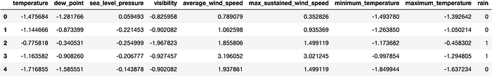
This example uses rainfall data publicly available from the National Oceanic and Atmospheric Administration (NOAA) [1]. This dataset contains weather measurements collected over a 50- year period at a site location in Bellevue, Nebraska. It contains eight features: temperature, dew point, sea-level pressure, visibility, average wind speed, max sustained wind-speed, minimum temperature, and maximum temperature. The dependent variable is rain: 0 indicates it did not rain, 1 indicates it did rain on that day.
The dataset contains 18,159 daily readings of which 5,698 are rain (1) and the remaining 12,461 are no rain (0).
Preview of Rainfall Data:
Exploring the Data:
For the purposes of adding drift, we divided the dataset using a 50/50 train test split. The training dataset consisted of the first 9,000 samples, and the test dataset consisted of the latter 9,000. Concept and data drift were synthetically introduced to the test dataset using a simple feature swapping method, as described in Souza et al. [1]. Drift starts in timestamp 12,000 and persists through the rest of the dataset.
We trained a K-neighbors classifier with k=10 on the training data to predict ‘rain’ and achieved an average test accuracy score of 76%. After injecting drift into the test data, we applied the same classifier to compare its performance. When applying the same classifier to data containing drift, the accuracy of the model drops to an average score of 67%. The plot below compares the accuracy using test data. This confirms the presence of concept drift.

Apply Drift Detectors
We first read in the datasets, the original dataset and the dataset containing concept drift so we can compare performance. We split into train and test sets. Drift is only injected into the test data set. We apply a K-neighbors classifier to predict rainfall.
from sklearn.neighbors import KNeighborsClassifier
from sklearn.model_selection import train_test_split
from menelaus.datasets import fetch_rainfall_data
import pandas as pd
import numpy as np# read in data
df = fetch_rainfall_data()# train test split
X_train, X_test, y_train, y_test = train_test_split(
     df.iloc[:,:-1], df.iloc[:,-1], test_size=0.5,
     random_state=42,     shuffle = False
)# apply classifier
knn = KNeighborsClassifier(n_neighbors=10)
knn.fit(X_train,y_train)# get running accuracy from classifier to compare performance
acc_orig = np.cumsum(knn.predict(X_test) == y_test)
acc_orig = acc_orig / np.arange(1, 1 + len(acc_orig))
We set up the drift detector ADWIN and run the detector. If ADWIN detects drift, it recommends a new retraining window for the model, which should contain the new concept.
The aim is to adapt the model to the new concept so that it can stay resilient to drift. In this example, we perform retraining.
from menelaus.concept_drift import ADWINAccuracy
adwin = ADWINAccuracy()# Set up DF to record results.
status = pd.DataFrame(columns=["index", "y_true", "y_pred", "drift_detected"])
rec_list = []# run ADWIN
for i in range(len(X_train), len(df)):
     x = X_test.loc[[i]]
     y_pred = int(knn.predict(x))
     y_true = int(y_test.loc[[i]])
     adwin.update(y_true, y_pred)
     status.loc[i] = [i, y_true, y_pred, adwin.drift_state]# If drift is detected, examine the window and retrain.
     if adwin.drift_state == "drift":
          retrain_start = adwin.retraining_recs[0] + len(X_train)
          retrain_end = adwin.retraining_recs[1] + len(X_train)
          rec_list.append([retrain_start, retrain_end])          # The retraining recommendations produced here
          # correspond to the samples which belong to ADWIN's
          # new, smaller window, after drift is detected.
          # If retraining is not desired, omit the next four lines.
          X_train_new = X_test.loc[retrain_start:retrain_end,]
          y_train_new = y_test.loc[retrain_start:retrain_end,]
          knn = KNeighborsClassifier(n_neighbors=10)
          knn.fit(X_train_new, y_train_new)status['original_accuracy'] = acc_orig
status['accuracy'] = np.cumsum(status.y_true == status.y_pred)
status['accuracy'] = status['accuracy'] / np.cumsum(np.repeat(1,
     status.shape[0]))
Visualize Results
The below code plots the performance of the K-neighbors classifier and compares using the retraining recommendations versus not using them.
import matplotlib.pyplot as plt## Plotting ##
plt.figure(figsize=(16, 9))
plt.plot("index", "original_accuracy", data=status,
     label="Original Accuracy")
plt.plot("index", "accuracy", data=status,
     label="Retrain Accuracy")
plt.grid(False, axis="x")
plt.xticks(fontsize=16)
plt.yticks(fontsize=16)
plt.title("ADWIN Results: Accuracy", fontsize=22)
plt.ylabel("Value", fontsize=22)
plt.xlabel("Index", fontsize=22)
ylims = [0, 1.1]
plt.ylim(ylims)
plt.axvspan(12000, len(df), alpha=0.2, label="Drift Induction Window")# Draw red lines that indicate where drift was detected
plt.vlines(
     x=status.loc[status["drift_detected"] == "drift"]["index"],
     ymin=ylims[0],
     ymax=ylims[1],
     label="Drift Detected",
     color="red",
)# Create a list of lines that indicate the retraining windows.
# Space them evenly, vertically.
rec_list = pd.DataFrame(rec_list)
rec_list["y_val"] = np.linspace(
     start=0.05 * (ylims[1] - ylims[0]) + ylims[0],
     stop=0.2 * ylims[1],
     num=len(rec_list),
)# Draw green lines that indicate where retraining occurred
plt.hlines(
     y=rec_list["y_val"],
     xmin=rec_list[0],
     xmax=rec_list[1],
     color="green",
     label="Retraining Windows",
)plt.legend(loc='lower right', fontsize='x-large')
plt.show()
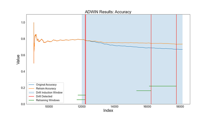
The indices included in the retraining recommendations are shown in green. The orange line indicates the accuracy when retraining using ADWIN’s recommendations. ADWIN successfully identifies drift and maintains the performance of the classifier.
Limitations of Concept Drift Detectors
As with any field of research, limitations and tradeoffs exist. A concept drift detector that monitors model performance alone, e.g. accuracy, will not be able to identify the features of the data set that contain drift. If you are interested in determining where drift is occurring, it is recommended to pair a concept drift detector with a data drift detector capable of identifying specific features containing drift.
Every detector has various settings and parameters that control how often it alarms to drift. As the true occurrence of drift is rarely known in real data, it can be challenging to determine the best combination of settings within a given environment. To identify the optimal parameters, it is necessary to bring in domain knowledge to consider the meaning of drift alarms within the context of the use case.
Two important tradeoffs users should be aware of are between sensitivity and computational speed, and between sensitivity and the false alarm rate. Checking for drift with every new sample calls for more computation, which may be a problem in settings with large volumes of data. Additionally, selecting parameters that result in the detector being highly sensitive to drift can result in a greater number of false alarms. Some detectors have theoretical guarantees for that rate, and each detector might call for a different tradeoff.
Resources to Learn More:
Find our package at the following links. Our team welcomes any feedback and opportunities for collaboration.
To gain a deeper understanding of concept drift and the techniques used by a variety of algorithms to detect it, we recommend reading the 2019 Lu et al. survey paper Learning under Concept Drift: A Review [2].
To learn more about the MITRE corporation, visit the website here.
Additional Details on Algorithms in the Menelaus library:
DDM
DDM monitors the minimum probability of a classification error. If this probability and its standard deviation exceed a specific threshold, a user is alerted to drift. It relies on the assumption that a classifier’s error rate is binomially distributed. DDM is intended for use with a binary classifier [4].
EDDM
EDDM monitors the distance between two classification errors for each element in the data stream. If this distance and its standard deviation exceed a certain threshold, a user is alerted to drift. EDDM is intended for use with a binary classifier [5].
LFR
LFR monitors a classifier’s true positive rate, true negative rate, negative predictive value, and positive predictive value to detect drift. It relies on the assumption that a significant change in any of these rates implies a change in the joint distribution of the features with the label. A significant drift in any of the four rates leads to an alarm that the distribution of the given rate at time T-1 is not equal to the distribution of the rate at time T. Monte Carlo simulations are used to derive empirical distributions of the rate. LFR assumes the target variable is binary [6].
STEPD
STEPD is a streaming drift detection algorithm intended to monitor the accuracy of an online binary classifier. When paired with an online classifier trained on every new sample, it can determine whether the classifier should be re-trained on a set of samples from a new concept [7].
MD3
MD3 is a semi-supervised algorithm. It tracks the number of samples in a classifier’s region of uncertainty, the margin. It warns of drift when the density of the classifier’s margin changes but it only alerts to drift when this change is associated with a drop in the classifier’s accuracy [8].
ADWIN
ADWIN is a change detection algorithm which monitors the running mean and variance of a given value via an adaptive sliding window. The window expands with time as the statistic remains consistent. When drift is detected, the window shrinks to only data which is consistent with the new regime. Since ADWIN can be applied to arbitrary values, it can be applied as a concept drift detection algorithm by monitoring e.g. accuracy or error rate. Menelaus includes an API to apply ADWIN to either arbitrary values (operating as a change detector) or to accuracy (operating as a concept drift detector) [9].
Page Hinkley
Page Hinkley is a univariate change detection algorithm, designed to detect changes in a sequential Gaussian signal using streaming data. The test statistic monitors how far the current observation is from the running mean of all previously encountered observations, while weighting it by a sensitivity parameter. The detector alarms when the difference between the maximum or minimum PH statistic encountered is larger than the cumulative PH statistic threshold [10].
CUSUM
CUSUM is an algorithm from the field of statistical process control. It is intended for streaming data and tests for changes in the mean of a time series by calculating a moving average over recent observations. CUSUM can be applied to the mean of a feature variable of interest or can track a single model performance metric [11].
References:
- V. Souza, D. M. dos Reis, A. G. Maletzke, and G. E. Batista, “Challenges in benchmarking stream learning algorithms with real-world data,” Data Mining and Knowledge Discovery, vol. 34, no. 6, pp. 1805–1858, 2020.
- J. Lu, A. Liu, F. Dong, F. Gu, J. Gama, and G. Zhang, “Learning under Concept Drift: A Review,” IEEE Transactions on Knowledge and Data Engineering, vol. 31, no. 12, pp. 2346–2363, 2019, doi: 10.1109/TKDE.2018.2876857.
- L. Nicholl, T. Schill, I. Lindsay, A. Srivastava, K. P. McNamara, and S. Jarmale, Menelaus. The MITRE Corporation, 2022. [Online]. Available: https://github.com/mitre/menelaus
- J. Gama, P. Medas, G. Castillo, and P. Rodrigues, “Learning with drift detection,” in Brazilian symposium on artificial intelligence, 2004, pp. 286–295.
- M. Baena-Garcıa, J. del Campo-Ávila, R. Fidalgo, A. Bifet, R. Gavalda, and R. Morales-Bueno, “Early drift detection method,” in Fourth international workshop on knowledge discovery from data streams, 2006, vol. 6, pp. 77–86.
- H. Wang and Z. Abraham, “Concept drift detection for streaming data,” in 2015 international joint conference on neural networks (IJCNN), 2015, pp. 1–9.
- K. Nishida and K. Yamauchi, “Detecting concept drift using statistical testing,” in International conference on discovery science, 2007, pp. 264–269.
- T. S. Sethi and M. Kantardzic, “On the reliable detection of concept drift from streaming unlabeled data,” Expert Systems with Applications, vol. 82, pp. 77–99, 2017.
- A. Bifet and R. Gavalda, “Learning from time-changing data with adaptive windowing,” in Proceedings of the 2007 SIAM international conference on data mining, 2007, pp. 443–448.
- D. V. Hinkley, “Inference about the change-point from cumulative sum tests,” Biometrika, vol. 58, no. 3, pp. 509–523, 1971.
- E. S. Page, “Continuous inspection schemes,” Biometrika, vol. 41, no. 1/2, pp. 100–115, 1954.
Approved for Public Release; Distribution Unlimited. Public Release Case Number 22–3165 ©2022 The MITRE Corporation. ALL RIGHTS RESERVED.